10. Applications of First order ODEs

First-order ordinary differential equations (ODEs) are crucial in modeling various real-world phenomena. In this section, we’ll explore five practical examples that illustrate the application of first-order ODEs in different fields. These examples are designed just to be aware of how basic concepts of first-order ODEs can be applied in real world scenarios.

1. Application 1: Chemical mixing

1.1. Example 1: Salt mixture

A tank with a capacity of 600 gallons initially contains 300 gallons of water with 150 pounds of salt dissolved in it. A salt solution containing 2 pounds of salt per gallon enters the tank at a rate of 4 gallons per minute. The mixture is stirred thoroughly, and a mixture with the same concentration exits the tank at a rate of 3 gallons per minute. Find the amount of salt in the tank when it overflows.

The above scenario can be expressed as in the image below.

Solution:

Inlet of salt solution - 4 gallons per minute

Outlet of salt solution - 3 gallons per minute

Step 1: Define Variables

- Let $S(t)$ represent the amount of salt (in pounds) in the tank at time $t$ (in minutes).

- Let $V(t)$ represent the volume of solution (in gallons) in the tank at time $t$ .

Step 2: Determine the Volume of Solution $V(t)$

Since the tank starts with 300 gallons and the net inflow rate is $4 \text{ gal/min} - 3 \text{ gal/min} = 1 \text{ gal/min}$ :

V(t) = 300 + t \text{ gallons}

The tank will overflow when $V(t) = 600$ gallons. Therefore, the time $T$ at which the tank overflows is:

600 = 300 + T \implies T = 300 \text{ minutes}

Step 3: Set Up the Differential Equation

The rate of change of salt in the tank is given by:

\frac{dS(t)}{dt} = \text{Rate In} - \text{Rate Out}

Rate In: The rate at which salt enters the tank is the concentration of the incoming solution multiplied by the rate at which it flows in:

\text{Rate In} = 2 \text{ lb/gal} \times 4 \text{ gal/min} = 8 \text{ lb/min}

Rate Out: The rate at which salt leaves the tank depends on the concentration of salt in the tank and the outflow rate. The concentration in the tank at time $t$ is $\frac{S(t)}{V(t)}$ pounds per gallon:

\text{Rate Out} = \frac{S(t)}{V(t)} \times 3 \text{ gal/min} = \frac{3S(t)}{300 + t} \text{ lb/min}

Step 4: Formulate the Initial Value Problem

The differential equation governing the amount of salt in the tank is:

\frac{dS(t)}{dt} = 8 - \frac{3S(t)}{300 + t}

with the initial condition $S(0) = 150$ pounds.

2. Application 2: Population growth models

2.1. Example 1: Human Population growth

A town’s population grows at a rate proportional to its current size. Suppose the population increases by 2% per year. If the initial population at time $t = 0$ is 1000, find the population after 5 years.

Solution:

Step 1: Set Up the Differential Equation

The population growth can be modeled by:

\frac{dP}{dt} = kP

where $P(t)$ is the population at time $t$ and $k$ is the growth rate. Given $k = 0.02$ , the equation becomes:

\frac{dP}{dt} = 0.02P

The population growth is modeled by the differential equation $\frac{dP}{dt} = kP$ because existing people give birth to new ones, so the more people you have the more offspring are born. This means that as the population grows, the number of new births also increases, leading to faster population growth over time. The constant $k$ represents the growth rate, which is the average number of births per person per unit of time. This model reflects the idea that with more people, there are more offspring being born, resulting in exponential growth of the population.

Step 2: Solve the Differential Equation

Separate variables and integrate:

\frac{1}{P} \, dP = 0.02 \, dt

Integrating both sides:

\ln |P| = 0.02t + C

Exponentiate:

P(t) = C_1 e^{0.02t}

Step 3: Apply Initial Condition

Given $P(0) = 1000$ :

1000 = C_1 \implies P(t) = 1000 e^{0.02t}

Step 4: Calculate Population After 5 Years

P(5) = 1000 \times e^{0.1} \approx 1105

Answer: The population after 5 years will be approximately 1105 people.

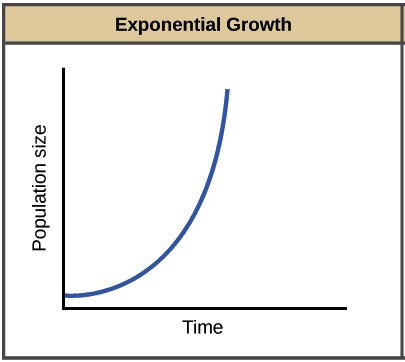
The below image shows how population size changes with time exponentially.

2.2. Example 2: Mosquito Population with Predation

In the absence of predators, the population of mosquitoes in a certain area increases at a rate proportional to its population and doubles every three weeks. Initially, there were 250,000 mosquitoes. However, a flock of birds arrives and eats 80,000 mosquitoes per week. We want to determine the number of mosquitoes remaining after two weeks.

Solution:

1. Define the Population Function:

Let $M(t)$ be the number of mosquitoes at time $t$ weeks. The population growth is exponential, and given that the population doubles every three weeks, the growth rate can be expressed as:

M(t) = M(0) \times 2^{\frac{t}{3}}

This can be rewritten using natural logarithms as:

M(t) = M(0) \times e^{\frac{1}{3} \log(2) \cdot t}

The growth rate per week is $\frac{1}{3} \log(2)$ .

2. Incorporate Predation:

The birds eat 80,000 mosquitoes per week. This reduces the growth rate, leading to a differential equation that governs the population:

\frac{dM}{dt} = \frac{1}{3} \log(2) M(t) - 80,000

Initially, $M(0) = 250,000$ .

3. Formulate the Initial Value Problem:

The problem becomes solving the following initial value problem:

\frac{dM}{dt} - \frac{1}{3} \log(2) M(t) = -80,000, \quad M(0) = 250,000

4. By solving the above results in approximately 193,500 mosquitoes remaining after two weeks.

2.3. Example 3: Logistic Population Model

When a population grows without any constraints, it follows an exponential growth model. However, in reality, limited resources lead to competition, which slows down the growth rate as the population increases. This can be modeled using the logistic equation:

\frac{dP}{dt} = rP - aP^2

In this equation:

- The term $rP$ represents the natural growth of the population, similar to the exponential model.

- The term $-aP^2$ accounts for the negative effects of competition for resources. As the population grows, individuals compete more intensely, leading to outcomes like wars, starvation, and increased deaths, which slow down population growth. The coefficient $a$ quantifies the intensity of competition. The term is quadratic ( $P^2$ ) because competition involves interactions between pairs of individuals, making its effect on growth proportional to the square of the population size.

Phase Line Portrait for the Logistic Equation

To analyze the behavior of the population over time, we can create a phase line portrait. The phase line helps visualize the stability of equilibrium points (where $\frac{dP}{dt} = 0$ ) and understand how the population changes.

1. Finding Equilibrium Points:

Setting $\frac{dP}{dt} = 0$ gives us the equilibrium points:

rP - aP^2 = 0

Factoring the equation:

P(r - aP) = 0

This results in two equilibrium points:

- $P = 0$ (extinction)

- $P = \frac{r}{a}$ (carrying capacity)

2. Phase Line Analysis:

- For $P < 0$ : The population is not physically meaningful.

- For $0 < P < \frac{r}{a}$ : $\frac{dP}{dt} > 0$ , meaning the population increases.

- For $P = \frac{r}{a}$ : $\frac{dP}{dt} = 0$ , indicating a stable equilibrium (carrying capacity).

- For $P > \frac{r}{a}$ : $\frac{dP}{dt} < 0$ , meaning the population decreases.

3. Phase Line Portrait:

The phase line is represented as follows:

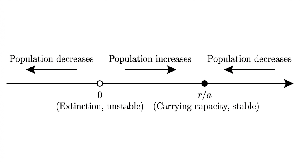
- Arrows pointing away from $P = 0$ indicate that any population slightly above zero will grow towards the carrying capacity.

- Arrows pointing towards $P = \frac{r}{a}$ indicate that populations above the carrying capacity will decrease to this equilibrium point.

4. Interpretation of the Phase Line:

- Sudden Drop in Population (e.g., Pandemic):

- If a pandemic causes a sudden drop in the population below the carrying capacity $\left(\frac{r}{a}\right)$ , the phase line indicates that the population will still grow back towards the carrying capacity over time. This shows that the carrying capacity is a stable equilibrium, so the population tends to return to this level even after disturbances.

- Sudden Increase in Population (e.g., Immigration):

- If there is a sudden influx of people (e.g., due to immigration) that pushes the population above the carrying capacity, the phase line shows that the population will decrease back towards the carrying capacity. The carrying capacity acts as a stable point that the population naturally converges to over time.

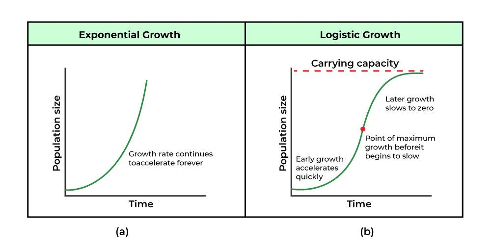
In both scenarios, the population eventually stabilizes at the carrying capacity $\frac{r}{a}$ , demonstrating the resilience of the system to return to equilibrium despite temporary disruptions.

Below graphs show the exponential and logistic growth curves.

3. Application 3: Newton’s Law of Cooling

3.1. Example 1: Cooling of a Hot Object

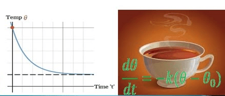
A hot cup of coffee at 90°C cools down in a room at 20°C. The cooling rate is proportional to the temperature difference between the coffee and the room. If the coffee cools to 60°C in 10 minutes, what will its temperature be after 20 minutes?

Solution:

Step 1: Set Up the Differential Equation

According to Newton’s Law:

\frac{dT}{dt} = -k(T - 20)

As the coffee cools down and the temperature difference decreases, the rate of cooling also slows down. This is why, for example, a very hot object cools rapidly at first but then slows down as it approaches room temperature.

The equation $\frac{dT}{dt} = -k(T - 20)$ captures this behavior mathematically. Here, $\frac{dT}{dt}$ represents the rate of change of temperature over time. The negative sign indicates that the temperature is decreasing.

The term (T−20)(T - 20)(T−20) represents the difference between the coffee's temperature TTT and the room temperature (20°C). Since the rate of cooling is proportional to this difference, the equation reflects that a larger difference leads to a faster cooling rate.

Step 2: Solve the Differential Equation

Separate variables and integrate:

\frac{1}{T - 20} \, dT = -k \, dt

Integrating both sides:

\ln |T - 20| = -kt + C

Exponentiate:

T(t) = 20 + C_1 e^{-kt}

Step 3: Apply Initial Condition

Given $T(0) = 90$ :

90 = 20 + C_1 \implies C_1 = 70

Step 4: Determine $k$

Given $T(10) = 60$ :

60 = 20 + 70 e^{-10k} \implies k \approx 0.0488

Step 5: Calculate Temperature After 20 Minutes

T(20) = 20 + 70 e^{-0.976} \approx 46.3

Answer: The temperature after 20 minutes will be approximately 46.3°C.

4. Application 4: Radioactive Decay

Radioactive decay is a natural process by which an unstable atomic nucleus loses energy by emitting radiation. A classic example of this is the decay of Carbon-14 , which is used in radiocarbon dating to determine the age of archaeological artifacts. Carbon-14 is a radioactive isotope of carbon found in all living organisms. When an organism dies, it stops absorbing Carbon-14, and the existing ${14}^C$ starts to decay into Nitrogen-14 at a known rate, allowing scientists to estimate the time since the organism's death.

4.1. Example 1: Radioactive Decay and Carbon-14 Dating

A fossilized tree killed by a volcanic eruption was studied. The fossil contains 6.25% of the original amount of carbon-14 ( $C^{14}$ ) found in a living tree today. We need to estimate how long ago the volcanic eruption occurred. The half-life of carbon-14 is 5730 years.

Step 1: Understanding the Decay Formula

Radioactive decay is governed by the formula:

N(t) = N_0 \cdot \left(\frac{1}{2}\right)^{\frac{t}{T_{1/2}}}

Where:

- $N(t)$ is the remaining quantity of the substance at time $t$ .

- $N_0$ is the initial quantity of the substance.

- $T_{1/2}$ is the half-life of the substance.

- $t$ is the time elapsed.

Step 2: Apply Given Data

In this problem:

- $N(t) = 6.25\% = 0.0625 \times N_0$

- $N_0 = 100\%$

- $T_{1/2} = 5730$ years

We need to find $t$ , the time elapsed since the tree was fossilized.

Step 3: Set Up the Equation

Using the decay formula:

0.0625 \times N_0 = N_0 \cdot \left(\frac{1}{2}\right)^{\frac{t}{5730}}

We can cancel $N_0$ from both sides:

0.0625 = \left(\frac{1}{2}\right)^{\frac{t}{5730}}

Step 4: Solve for $t$

To solve for $t$ , take the natural logarithm on both sides:

\ln(0.0625) = \ln\left[\left(\frac{1}{2}\right)^{\frac{t}{5730}}\right]

Using the logarithm power rule $\ln(a^b) = b \ln(a)$ :

\ln(0.0625) = \frac{t}{5730} \cdot \ln\left(\frac{1}{2}\right)

Now solve for $t$ :

t = 5730 \cdot \frac{\ln(0.0625)}{\ln(0.5)}

Step 5: Calculate the Value of $t$

\ln(0.0625) \approx -2.7726

\ln(0.5) \approx -0.6931

Thus:

t = 5730 \cdot \frac{-2.7726}{-0.6931} \approx 5730 \cdot 4 = 22920 \text{ years}

The volcanic eruption that fossilized the tree occurred approximately 22,920 years ago, based on the decay of carbon-14 in the sample.

5. Application 5: Spring-Mass System

5.1. Example 1: Simple Harmonic Motion

A mass attached to a spring oscillates back and forth. If the displacement from equilibrium is small, the motion can be modeled by a first-order ODE. Given the initial velocity and displacement, find the displacement as a function of time.

Solution:

Step 1: Set Up the Differential Equation

The motion is modeled by:

\frac{dv}{dt} = -\frac{k}{m} x

where $x(t)$ is the displacement, $v(t)$ is the velocity, $k$ is the spring constant, and $m$ is the mass.

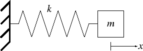
This equation is modeled using below laws ;

1. Hooke’s Law:

Hooke's Law states that the force exerted by a spring is proportional to the displacement $x$ from its equilibrium position:

F_{\text{spring}} = -kx

Here:

- $F_{\text{spring}}$ is the restoring force exerted by the spring.

- $k$ is the spring constant, which measures the stiffness of the spring.

- $x$ is the displacement from the equilibrium position.

- The negative sign indicates that the force is directed opposite to the displacement, trying to restore the mass to equilibrium.

2. Newton’s Second Law:

Newton's Second Law of Motion relates the net force acting on a mass to its acceleration:

F_{\text{net}} = ma

Here:

- $F_{\text{net}}$ is the total force acting on the mass.

- $m$ is the mass.

- $a$ is the acceleration, which can be expressed as the time derivative of velocity $v$ , i.e., $a = \frac{dv}{dt}$ .

3. Combining Hooke’s Law and Newton’s Second Law:

In the case of a mass attached to a spring, the only force acting on the mass (assuming no damping or external forces) is the restoring force from the spring. Therefore: $ma = -kx$

Substituting $a = \frac{dv}{dt}$ :

m \frac{dv}{dt} = -kx

Dividing both sides by $m$ gives the first-order ordinary differential equation:

\frac{dv}{dt} = -\frac{k}{m} x

This equation describes how the velocity of the mass changes over time due to the restoring force of the spring. The term $-\frac{k}{m} x$ indicates that the acceleration (and thus the change in velocity) is proportional to the displacement $x$ , but in the opposite direction, which is characteristic of oscillatory motion.

Given the initial conditions (initial velocity and displacement), the motion of the mass can be modeled by the differential equation:

\frac{dv}{dt} = -\frac{k}{m} x

Where:

- $x(t)$ is the displacement as a function of time.

- $v(t)$ is the velocity as a function of time.

- $k$ is the spring constant.

- $m$ is the mass.

Step 2: Solve the Differential Equation

Solve the system using initial conditions for displacement and velocity.

Step 3: Apply Initial Condition

Given initial conditions for velocity and displacement, solve for the constants.

Answer: The displacement $x(t)$ will oscillate sinusoidally, depending on the initial conditions.

6. Application 6: First-Order Kinetics

6.1. Example 1: Chemical Reaction Rate

In a chemical reaction, the concentration of a reactant decreases at a rate proportional to its current concentration. If the concentration drops from 1 M to 0.5 M in 10 minutes, how much will remain after 30 minutes?

Solution:

Step 1: Set Up the Differential Equation

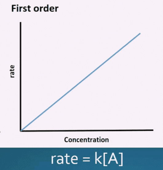
The reaction rate is modeled by:

\frac{dC}{dt} = -kC

where $C(t)$ is the concentration of the reactant.

In a first-order reaction, the rate at which the concentration C of the reactant decreases depends on how much of the reactant is present at that moment. This means that when the concentration is high, the reaction proceeds quickly; as the concentration decreases, the reaction slows down.

The negative sign indicates that the concentration C is decreasing over time. The constant kkk is the rate constant, which characterizes how quickly the reaction proceeds.

Step 2: Solve the Differential Equation

Separate variables and integrate:

\frac{1}{C} \, dC = -k \, dt

Integrating:

\ln |C| = -kt + C

Exponentiate:

C(t) = C_1 e^{-kt}

Step 3: Apply Initial Condition

Given $C(0) = 1$ :

1 = C_1 \implies C(t) = e^{-kt}

Step 4: Determine $k$

Given $C(10) = 0.5$ :

0.5 = e^{-10k} \implies k \approx 0.0693

Step 5: Calculate Remaining Concentration After 30 Minutes

C(30) \approx 0.125 \text{ M}

Answer: Approximately 0.125 M of the reactant will remain after 30 minutes.

7. Application 7 : Financial applications

7.1. Example 1: Saving for a College Fund

Imagine a parent wants to save for their child's college education. They decide to make continuous contributions to a savings account at a constant rate, with the account earning interest compounded continuously. The goal is to have a specific amount saved up by the time the child turns 18.

Let's say the parent wants to save $50,000 by the time their child turns 18. The savings account offers an interest rate of 4% per year, compounded continuously. The parent can contribute continuously at a rate of $P$ dollars per year.

1. Determine the Continuous Payment Rate $P$ :

Let $S(t)$ be the balance in the savings account at time $t$ years. The differential equation representing the growth of the savings account is:

\frac{dS}{dt} = 0.04S + P

The change in the savings account balance is due to the interest earned, represented by $0.04S$ , and the continuous annual payment $P$ .

Given that the target amount is $50,000 by the time the child turns 18, we impose the condition:

S(18) = 50,000

The initial condition is $S(0) = 0$ , assuming the account starts with no initial balance.

2. Solving the Differential Equation:

The differential equation is a nonhomogeneous linear equation, and we can solve it using an integrating factor. First, rewrite the equation in its standard form:

\frac{dS}{dt} - 0.04S = P

The integrating factor is $e^{-0.04t}$ , so the equation becomes:

\frac{d}{dt}\left(e^{-0.04t}S(t)\right) = Pe^{-0.04t}

Integrating both sides with respect to $t$ , we obtain:

e^{-0.04t}S(t) = \int Pe^{-0.04t} dt = -\frac{P}{0.04} e^{-0.04t} + C

Multiplying through by $e^{0.04t}$ gives:

S(t) = \frac{P}{0.04} + Ce^{0.04t}

To find $C$ , use the initial condition $S(0) = 0$ :

0 = \frac{P}{0.04} + C \Rightarrow C = -\frac{P}{0.04}

So the solution is:

S(t) = \frac{P}{0.04} \left(1 - e^{-0.04t}\right)

3. Finding $P$ to Reach the Target:

Now, we use the condition $S(18) = 50,000$ to find $P$ :

50,000 = \frac{P}{0.04} \left(1 - e^{-0.72}\right)

Simplifying:

P = 50,000 \times 0.04 \div \left(1 - e^{-0.72}\right)

This simplifies to approximately $P \approx 2,817$ dollars per year. The exact form is better left unsimplified as:

P = \frac{50,000 \times 0.04}{1 - e^{-0.72}}

Thus, the parent needs to save continuously at a rate of about $2,817 per year to reach the $50,000 goal by the time the child turns 18.

7.2. Example 2: Financing a Home

Suppose a homebuyer wants to purchase a house and has secured a loan to cover the cost. The loan has a fixed interest rate of 4% per year, compounded continuously. The buyer plans to make continuous payments on the loan at a constant rate and aims to pay off the loan completely in 10 years.

Question: If the buyer can afford to pay $1,200 per month continuously, how much can they borrow?

1. Define the Problem:

Let $B(t)$ be the balance of the loan at time $t$ years. The differential equation that governs the balance is:

\frac{dB}{dt} = 0.04B - P

where:

- $r = 0.04$ (interest rate per year)

- $P = 12 \times 1,200 = 14,400$ dollars per year (payment rate)

- The goal is to have the loan paid off in 10 years, so $B(10) = 0$ .

The term $0.04B$ represents the interest charged on the remaining loan balance $B$ at a rate of 4% per year.

2. Set Up the Initial-Value Problem:

The initial loan amount is $B(0) = B_I$ . The differential equation is:

\frac{dB}{dt} = 0.04B - 14,400

with the condition $B(10) = 0$ .

3. Solve the Differential Equation:

This is a nonhomogeneous linear differential equation. First, rewrite it in standard form:

\frac{dB}{dt} - 0.04B = -14,400

The integrating factor is $e^{-0.04t}$ , so multiply the entire equation by this factor:

\frac{d}{dt}\left(e^{-0.04t}B(t)\right) = -14,400e^{-0.04t}

Now, integrate both sides with respect to $t$ :

e^{-0.04t}B(t) = -14,400 \int e^{-0.04t} dt

The integral on the right side is:

e^{-0.04t}B(t) = \frac{-14,400}{-0.04}e^{-0.04t} + C

Simplifying:

e^{-0.04t}B(t) = 360,000e^{-0.04t} + C

Multiplying both sides by $e^{0.04t}$ :

B(t) = 360,000 + Ce^{0.04t}

To find $C$ , use the condition $B(10) = 0$ :

0 = 360,000 + Ce^{0.4} \Rightarrow C = -360,000e^{-0.4}

Therefore, the balance as a function of time is:

B(t) = 360,000(1 - e^{0.04(t - 10)})

4. Determine the Initial Loan Amount:

Now, find $B(0)$ , the initial loan amount:

B(0) = 360,000(1 - e^{-0.4})

This is approximately:

B(0) \approx 360,000 \times 0.3297 \approx 118,692 \text{ dollars}

Thus, the buyer can afford to borrow about $118,692 with continuous payments of $1,200 per month over 10 years.

This article is designed to help you understand the practical applications of first-order ordinary differential equations (ODEs) by exploring five real-world examples. Don’t worry if some of the scenarios seem unfamiliar or complex; the goal here is to build your understanding of how first-order ODEs work in different contexts. Focus on the mathematical processes, and over time, the real-world connections will become clearer.

Hope you're enjoying the ODE series; stay tuned for the next sections.