In the study of differential equations, graphical methods often provide a deeper understanding of solutions. One of the most useful graphical techniques is the phase-line portrait, particularly for autonomous equations. In this article, we'll explore phase-line portraits in detail, providing clear explanations and examples with graphs to illustrate the concepts.

1. What is a Phase-Line Portrait?

A phase-line portrait is a graphical representation of the solutions of an autonomous differential equation, which is an equation of the form:

\frac{dy}{dt} = g(y)

In a phase-line portrait, the behavior of the solutions is represented along a horizontal line, showing the direction of motion of the solution as time progresses. The key idea is to determine the sign of  g(y) \ at various points along the interval of interest. The sign of  g(y) \ indicates whether the solution is increasing or decreasing at that point.

Steps to Create a Phase-Line Portrait

1. Identify Critical Points:

   - Find all points where  g(y) = 0 These are the stationary points where the solution does not change over time.

   - Identify any points where  g(y) is undefined.

2. Determine the Sign of  g(y) :

   - For each subinterval between the critical points and points where g is undefined, determine whether  g(y) is positive or negative.

3. Draw the Phase-Line:

   - Mark the stationary points with dots (•) on the phase-line.

   - Use arrows to indicate the direction of motion in each subinterval:

     - A right arrow (-->) indicates  g(y) > 0 (the solution increases).

     - A left arrow (←) indicates  g(y) < 0 (the solution decreases).

4. Analyze the Stability:

   - Determine the stability of each stationary point:

- Stable Point: Solutions move towards this point over time. On a phase line, arrows point towards the stable point from both sides.

- Unstable Point: Solutions move away from this point over time. On a phase line, arrows point away from the unstable point on both sides.

- Semi stable Point: Solutions move towards this point from one side but away from it on the other side. On a phase line, arrows point towards the semi stable point from one side and away from it on the other side.

2. Examples and Graphical Illustrations

2.1. Example 1: A Simple Cubic Equation

 Differential Equation: 

 \frac{dy}{dt} = 4y - y^3

This equation tells us how the variable  y changes with respect to time  t.

 Step 1: Identify Critical Points

Critical points, also known as equilibrium or stationary points, are values of  y where the derivative \frac{dy}{dt} = 0. These points are important because they represent where  y stops changing either the system stays at this point or the direction of change reverses.

1. Set the equation equal to zero:

    4y - y^3 = 0 \

2. Factor the equation:

    y(4 - y^2) = 0 \

3. Factor further:

    y(2 - y)(2 + y) = 0 \

4. Solve for  y:

    y = 0, \quad y = 2, \quad y = -2 \

So, the critical points are  y = 0 \, \ y = 2 \, and \ y = -2 \.

 Step 2: Determine the Sign of  \frac{dy}{dt} \

Next, we need to understand the behavior of  y in different regions divided by these critical points. Specifically, we'll determine whether y is increasing or decreasing in each region.

The regions are:

• (-\infty, -2) \

• (-2, 0) \

• (0, 2) \

• (2, \infty) \

To check the sign of  \frac{dy}{dt} \ in each region, we substitute a value of y from within each interval into the original equation:

1. For  y in (-\infty, -2) \:

   - Choose  y = -3 .

   - Substitute  y = -3 into  \frac{dy}{dt} = 4y - y^3 \:

    \frac{dy}{dt} = 4(-3) - (-3)^3 = -12 - (-27) = 15  \

   - The sign is positive, so y is increasing in this region.

2. For y \in (-2, 0):

   - Choose  y = -1.

   - Substitute  y = -1:

     \frac{dy}{dt} = 4(-1) - (-1)^3 = -4 - (-1) = -3  \

   - The sign is negative, so y is decreasing in this region.

3. For y \in (0, 2):

   - Choose  y = 1.

   - Substitute  y = 1:

     \frac{dy}{dt} = 4(1) - (1)^3 = 4 - 1 = 3  \

   - The sign is positive, so  y \ is increasing in this region.

4. For  y \in (2, \infty) \:

   - Choose  y = 3 \.

   - Substitute  y = 3 \:

      \frac{dy}{dt} = 4(3) - (3)^3 = 12 - 27 = -15   \

   - The sign is negative, so  y \ is decreasing in this region.

 Step 3: Draw the Phase-Line

The phase line is a simple diagram that shows the direction of the change of  y \ in different intervals.

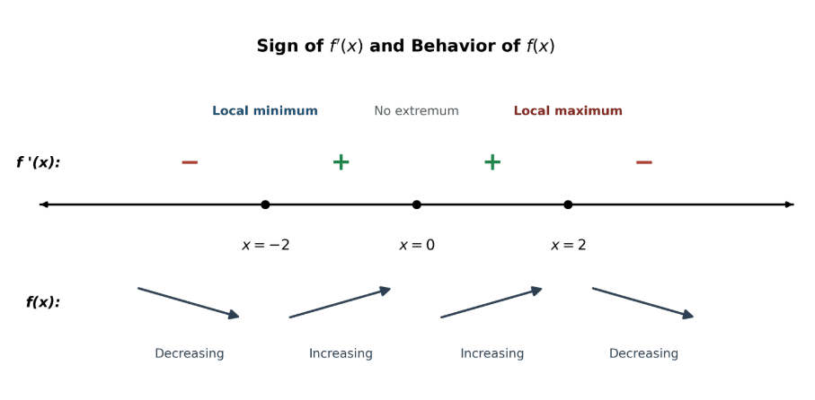
This shows:

-  y \ increases towards  -2 \ from the left.

-  y \ decreases towards  -2 \ from the right.

-  y \ increases towards  2 \ from the left.

-  y \ decreases towards  2 \ from the right.

 Step 4: Analysis of Stability

Now, let's analyze the stability of these critical points:

- Stable Points:  y = -2 \ and \ y = 2 \.

  - If  y \ starts slightly above or below  -2 \, it will eventually move towards  -2 \.

  - The same happens for  y = 2 \.

- Unstable Point:  y = 0 \.

  - If  y \ starts slightly above or below  0 \, it will move away from  0 \ over time.

 Interpretation:

- If the initial value of  y \ is less than  -2 \ or between  0 \ and  2 \,  y \ will eventually stabilize at  -2 \ or \ 2 \, respectively.

- If the initial value of  y \ is slightly off from  0 \,,  y \ will move away from  0 \, either towards  -2 \ or  \ 2 \.

The points  y = -2 \ and \  y = 2 \ are attractors, meaning the solutions tend to stabilize at these points. The point  y = 0 \ is a repeller, meaning that any small deviation from  y = 0 \ causes the solution to move away from it.

 Graphical Illustration

Differential Equation:  

 \frac{dy}{dt} = 4y - y^3 \

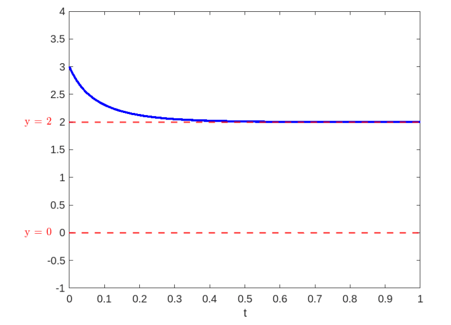
 Individual Graphs for Initial Values

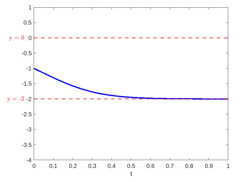
1. For  y(0) = -1 \:

   - Description:  

     This graph shows the trajectory of  y \ when starting at  -1 \. Given the differential equation,  y \ decreases when  y \ is between  -2 \ and  0 \. Therefore, starting from  -1 \, the graph demonstrates that  y \ moves towards the stable equilibrium at  -2 \, reflecting the decreasing behavior in this interval.

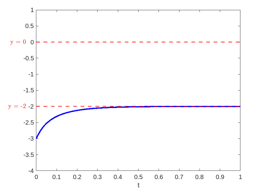
2. For  y(0) = -3 \:

   - Description:  

     This graph represents the trajectory starting at  -3 \. Since  y \ is less than  -2 \, the rate of change is positive, which means  y \ increases. This graph illustrates how  y \ moves towards the stable equilibrium at  -2 \, showing the increasing trend in this region.

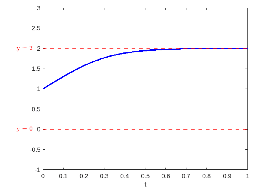
3. For  y(0) = 1 \:

   - Description:  

     This graph depicts the trajectory starting at  1 \. In this interval between  0 \ and \ 2 \,  y \ increases as indicated by the positive rate of change. The graph shows that  y \ approaches the stable equilibrium at  2 \.

4. For  y(0) = 3 \:

   - Description:  

     This graph illustrates the trajectory starting at  3 \. Since  y \ is greater than  2 \, the rate of change is negative, so  y \ decreases. The graph demonstrates how  y \ moves towards the stable equilibrium at  2 \.

 Final Plot with All Trajectories

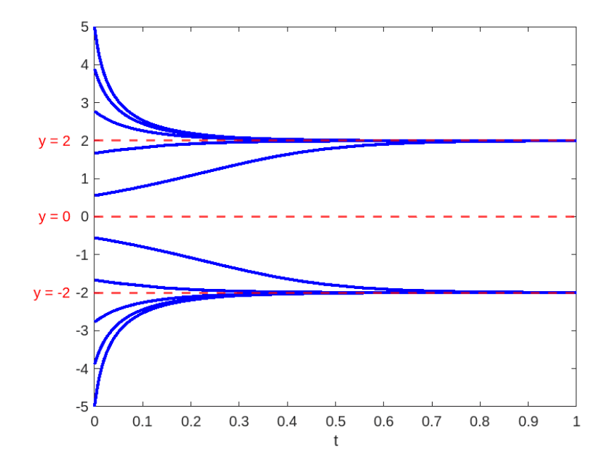
Description:  

The final plot combines all the individual trajectories starting from the initial values  y(0) = -5, -3, -1, 1, 3 \. This comprehensive plot visually represents the behavior of the solution curves over time, showing how each trajectory moves towards the critical points. The horizontal dashed lines represent the critical points  y = -2 \,  \ y = 0 \, and \ y = 2 \. The trajectories illustrate the stability of  y = -2 \ and \ y = 2 \ (attractors) and the instability of  y = 0 \ (repeller).

 Matlab Code to Generate the Final Plot:

%Choose 10 initial values y(0) between -5 and 5

c = linspace(-5, 5 , 10);

%Range for t axis

x = [0 1;

critical_points = [-2, 0, 2;

f = @(t,y) 4*y - y^3;

%Solve IVP for each initial value and plot them

for a = c

    disp(a);

    [t,yval = ode15s(f, x, a);

    plot(t, yval, 'Color', [0, 0, 1, 'LineWidth',2)

    xlabel('t')

    ylabel('y', 'Rotation',0)

    hold on

end

%Plot horizontal asymptote lines for each critical point

for p = critical_points

    yline(p,'--', 'LineWidth', 1.5, 'Color', [1, 0, 0);

end

hold off

This MATLAB code generates the plot by solving the initial value problem for various starting points and plotting the trajectories along with the critical points.

If you like more exploration on plotting these types of graphs can start with the above MATLAB code and proceed in plotting various graphs to identify their behavior.

2.2. Example 2: A Quadratic Equation

\frac{dx}{dt} = x(2 - x)(4 - x)^2\

 Step 1: Identify Critical Points

Critical points are the values of  x \ where \frac{dx}{dt} = 0\. These occur where any of the factors in the equation equals zero.

1. Set the equation equal to zero:

      x(2 - x)(4 - x)^2 = 0   \

2. Solve for  x \:

   -  x = 0 \

   -  2 - x = 0 \ gives  x = 2 \

   -  4 - x = 0 \ gives  x = 4 \

So, the critical points are  x = 0 \,  x = 2 \, and \ x = 4 \.

 Step 2: Determine the Sign of \frac{dx}{dt}\

To understand the behavior of  x \ in different intervals, we need to determine whether  \frac{dx}{dt} \ is positive or negative in each interval defined by the critical points. The intervals are:

-  (-\infty, 0) \

-  (0, 2) \

-  (2, 4) \

-  (4, \infty) \

We will substitute a value of  x \ from each interval into the equation to check the sign of  \frac{dx}{dt} \.

1. For  x \in (-\infty, 0) \:

   - Choose  x = -1 \.

   - Substitute  x = -1 \ into  \frac{dx}{dt} = x(2 - x)(4 - x)^2 \:

      \frac{dx}{dt} = (-1)(2 - (-1))(4 - (-1))^2 = (-1)(3)(5)^2 = -75   \

   - The sign is negative, so  x \ is decreasing in this region.

2. For  x \in (0, 2) \:

   - Choose  x = 1 \.

   - Substitute  x = 1 \:

      \frac{dx}{dt} = (1)(2 - 1)(4 - 1)^2 = (1)(1)(3)^2 = 9   \

   - The sign is positive, so  x \ is increasing in this region.

3. For  x \in (2, 4) \:

   - Choose  x = 3 \.

   - Substitute  x = 3 \:

      \frac{dx}{dt} = (3)(2 - 3)(4 - 3)^2 = (3)(-1)(1)^2 = -3   \

   - The sign is negative, so  x \ is decreasing in this region.

4. For  x \in (4, \infty) \:

   - Choose  x = 5 \.

   - Substitute  x = 5 \:

   \frac{dx}{dt} = (5)(2 - 5)(4 - 5)^2 = (5)(-3)(-1)^2 = -15\

   - The sign is negative, so  x \ is also decreasing in this region.

 Step 3: Draw the Phase-Line

Now that we know the signs in each interval, we can draw the phase line:

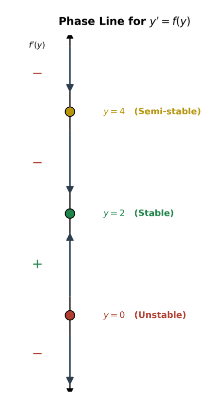
 Analysis:

- Stable Points:  x = 2 \,  \,x = 4 \.

  - If  x \ starts slightly above or below  2 \, it will move towards  2 \.

  - If  x \ starts slightly above or below  4 \, it will move towards  4 \.

- Unstable Point:  x = 0 \.

  - If  x \ starts slightly above  0 \, it will move away from  0 \.

Graphical Illustration:

Final Plot with trajectories

The final plot provides a comprehensive view of the system described by the differential equation \frac{dx}{dt} = x(2 - x)(4 - x)^2\. It illustrates how the system's behavior varies with different initial conditions. The plot features horizontal dashed lines at x = 0\, x = 2\, and \, x = 4\, marking the critical points where the rate of change \frac{dx}{dt}\ is zero. The trajectories show how x evolves over time:

- For initial values less than 0\,, x\ decreases and moves away from x = 0\, reflecting the negative rate of change in this region.

- For initial values between 0 \textrm{ and } 2, x increases towards x = 2\, as indicated by the positive rate of change.

- For initial values between 2 \textrm{ and } 4, xdecreases towards x = 2\, demonstrating a negative rate of change in this interval.

- For initial values greater than 4\,, x\ decreases towards x = 4\, also showing a negative rate of change.

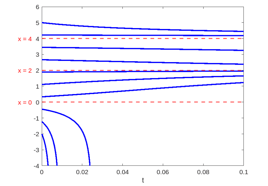
The plot effectively demonstrates the stability of the critical points x = 2 and x = 4 (stable points) and the instability of x = 0\ (unstable point), providing a clear visual representation of the system's dynamics.

The article continues: Phase-Line Portraits for Autonomous Equations II