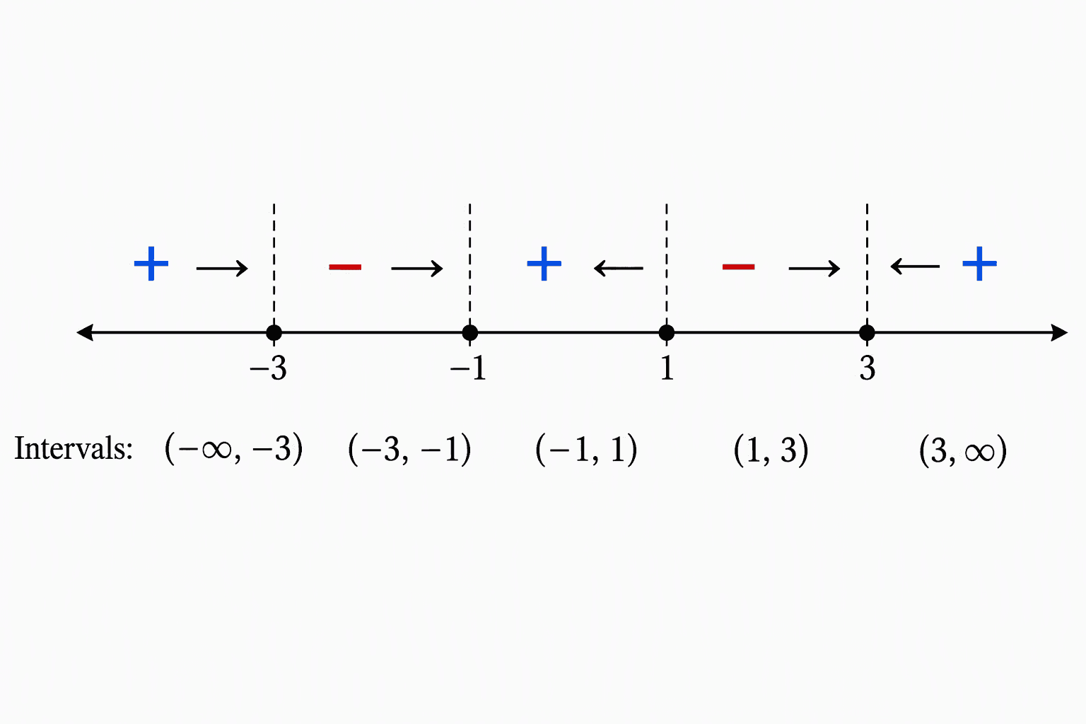
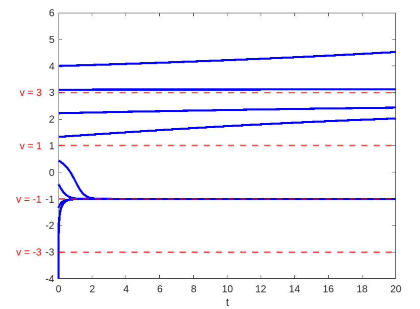
The final plot provides a comprehensive view of the system described by the differential equation \frac{dv}{dt} = \frac{(v^2 - 1)(v - 3)^2}{(v^2 + 1)(v + 3)^2}. It illustrates the system's behavior with various initial conditions. The plot features horizontal dashed lines at v = -1, v = 1, and v = 3, marking the critical points where the rate of change \frac{dv}{dt} is zero. The trajectories reveal how v evolves over time:
- For initial values less than -3, v decreases further, indicating a negative rate of change in this region.
- For initial values between -3 and -1, v increases towards v = -1, showing a positive rate of change.
- For initial values between -1 and 1, v decreases away from v = -1 and moves towards v = 1, reflecting a negative rate of change.
- For initial values between 1 and 3, v increases towards v = 3, indicating a positive rate of change.
- For initial values greater than 3, v decreases as it moves away from v = 3, showing a negative rate of change.
This plot effectively illustrates the complex behavior of the system, highlighting the stability of v = -1\ and the instability of v = 1\ and \ v = 3\.
1.2. Example 4: Linear Differential Equation
Equation:
\frac{dy}{dt} = y - 3\
Step 1: Identify Critical Points
- Set y - 3 = 0 \.
- Critical point: y = 3 \.
Step 2: Determine the Sign of g(y) \
- For y < 3 \,, g(y) = y - 3 < 0 \.
- For y > 3 \,, g(y) = y - 3 > 0 .
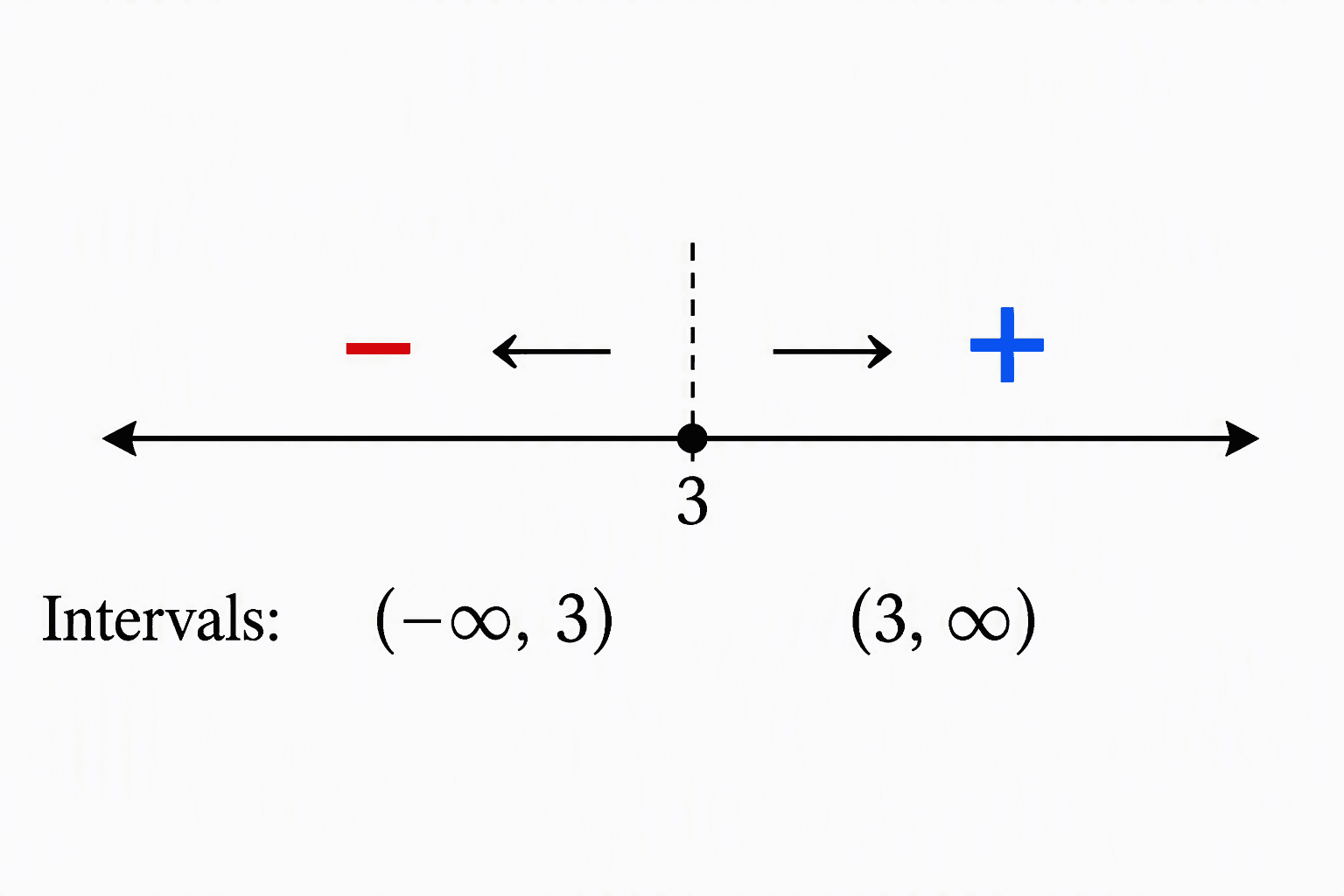
Step 3: Draw the Phase-Line
Analysis:
- Stable Point: y = 3 \.
Graphical Illustration:
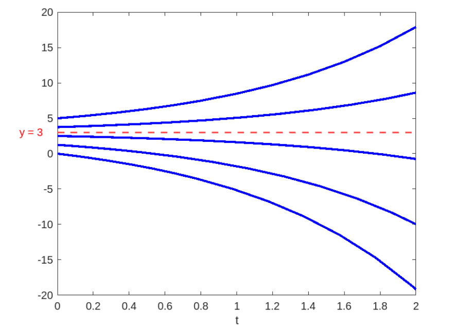
The final plot provides a clear depiction of the system governed by the differential equation \frac{dy}{dt} = y - 3. It demonstrates how the behavior of y varies with different initial conditions. The plot features a horizontal dashed line at y = 3, marking the critical point where the rate of change \frac{dy}{dt} is zero. The trajectories reveal how y evolves over time:
- For initial values less than 3, y increases towards y = 3, indicating that y is growing in this region and moving towards the stable point.
- For initial values greater than 3, y decreases towards y = 3, showing that y is decreasing and also moving towards the stable point.
This plot effectively illustrates the stability of the critical point y = 3, where solutions converge to this value regardless of whether the initial condition is above or below 3.
1.3. Example 5: Rational Function
Equation:
\frac{dy}{dt} = \frac{y^2 - 4}{y^2 + 1}
Step 1: Identify Critical Points
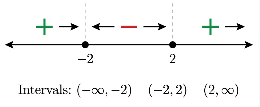
- Set \frac{y^2 - 4}{y^2 + 1} = 0.
- Critical points: y = \pm 2.
Step 2: Determine the Sign of g(y)
- For y < -2, g(y) = \frac{y^2 - 4}{y^2 + 1} > 0.
- For -2 < y < 2, g(y) = \frac{y^2 - 4}{y^2 + 1} < 0.
- For y > 2, g(y) = \frac{y^2 - 4}{y^2 + 1} > 0.
Step 3: Draw the Phase-Line
Analysis:
- Stable Points: y = \pm 2 \ (both are semi stable).
Graphical Illustration:
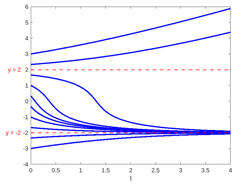
The final plot provides a detailed view of the system described by the differential equation \frac{dy}{dt} = \frac{y^2 - 4}{y^2 + 1}. It shows how the behavior of y varies with different initial conditions. The plot features horizontal dashed lines at y = -2 and y = 2, marking the critical points where the rate of change \frac{dy}{dt} is zero. The trajectories illustrate how y evolves over time:
- For initial values less than -2, y increases towards y = -2, reflecting a positive rate of change in this region.
- For initial values between -2 and 2, y decreases towards y = -2 or increases towards y = 2, showing a negative rate of change.
- For initial values greater than 2, y increases towards y = 2, indicating a positive rate of change.
This plot effectively demonstrates the semistable nature of the critical points y = \pm 2\, where trajectories exhibit different behaviors based on the direction of approach.
1.4. Example 6: Higher-Degree Polynomial
Equation:
\frac{dy}{dt} = y^3 - 3y
Step 1: Identify Critical Points
- Set y^3 - 3y = 0.
- Factor: y(y^2 - 3) = 0.
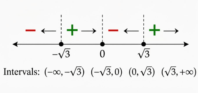
- Critical points: y = 0, y = \pm \sqrt{3}.
Step 2: Determine the Sign of g(y)
- For y < -\sqrt{3}, g(y) = y^3 - 3y > 0.
- For -\sqrt{3} < y < 0, g(y) = y^3 - 3y < 0.
- For 0 < y < \sqrt{3}, g(y) = y^3 - 3y < 0.
- For y > \sqrt{3}, g(y) = y^3 - 3y > 0.
Step 3: Draw the Phase-Line
Analysis:
- Stable Points: y = \pm \sqrt{3}.
- Unstable Point: y = 0.
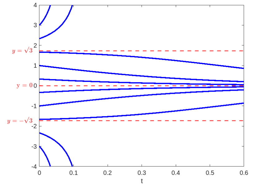
Graphical Illustration: The final plot offers a comprehensive view of the system governed by the differential equation \frac{dy}{dt} = y^3 - 3y. It illustrates how y evolves with different initial conditions. The plot features horizontal dashed lines at y = -\sqrt{3}, y = 0, and y = \sqrt{3}, marking the critical points where the rate of change \frac{dy}{dt} is zero. The trajectories provide insight into the system's behavior:
- For initial values less than -\sqrt{3}, y increases towards y = -\sqrt{3}, reflecting a positive rate of change in this region.
- For initial values between -\sqrt{3} and 0, y decreases towards y = -\sqrt{3}, showing a negative rate of change.
- For initial values between 0 and \sqrt{3}, y decreases towards y = 0 and increases towards y = \sqrt{3}, indicating a negative rate of change.
- For initial values greater than \sqrt{3}, y increases towards y = \sqrt{3}, reflecting a positive rate of change.
This plot effectively demonstrates the stability characteristics of the critical points y = \pm \sqrt{3} as stable points and y = 0 as an unstable point. The trajectories illustrate how solutions behave in different intervals around these critical points.
1.5. Example 7: Logarithmic Function
Equation:
\frac{dy}{dt} = \ln(y) - 1
Step 1: Identify Critical Points
- Set \ln(y) - 1 = 0.
- Critical point: y = e.
Step 2: Determine the Sign of g(y)
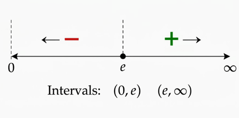
- For y < e, g(y) = \ln(y) - 1 < 0.
- For y > e, g(y) = \ln(y) - 1 > 0.
Step 3: Draw the Phase-Line
Analysis:
- Stable Point: y = e.
Graphical Illustration:
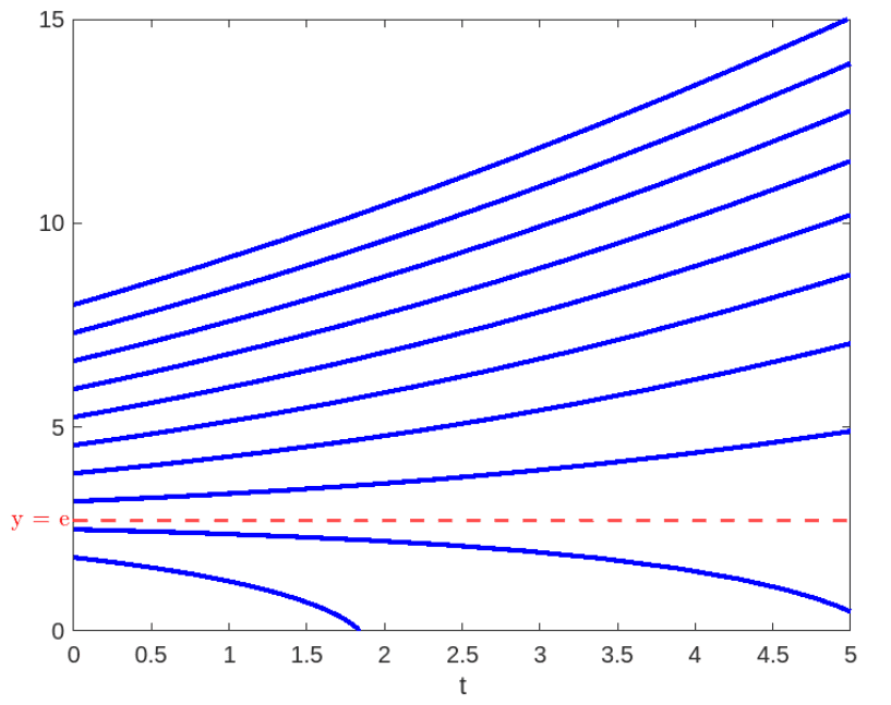
The final plot provides a clear visualization of the system described by the differential equation \frac{dy}{dt} = \ln(y) - 1. It demonstrates how y changes with various initial conditions. The plot includes a horizontal dashed line at y = e, marking the critical point where the rate of change \frac{dy}{dt} is zero. The trajectories reveal:
- For initial values less than e, y decreases, indicating that \frac{dy}{dt} is negative in this region.
- For initial values greater than e, y increases, showing a positive rate of change.
This plot effectively illustrates the stability of the critical point y = e. The trajectories converge towards y = e from both sides, highlighting that y = e is a stable point.
1.6. Example 8: Trigonometric Function
Equation:
\frac{dy}{dt} = \sin(y)
Step 1: Identify Critical Points
- Set \sin(y) = 0.
- Critical points: y = n\pi, where n
Step 2: Determine the Sign of g(y)
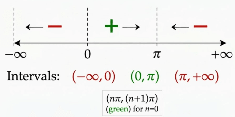
- For n\pi < y < (n+1)\pi, g(y) = \sin(y) oscillates between positive and negative values.
Step 3: Draw the Phase-Line
Analysis:
- Stable Points: y = n\pi (semistable points).
Graphical Illustration:
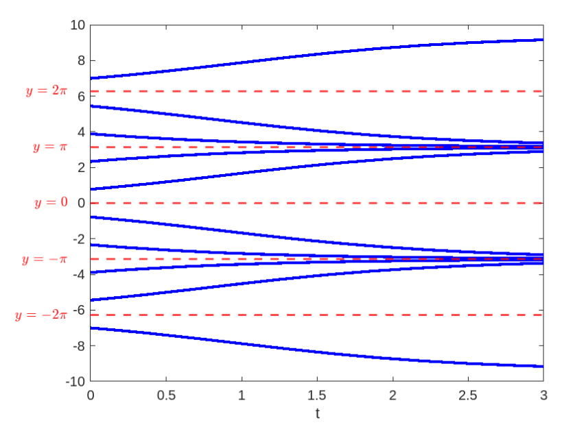
The final plot for the differential equation \frac{dy}{dt} = \sin(y) visually represents the system's dynamics over different intervals. The horizontal dashed lines indicate the critical points where \sin(y) = 0, specifically at y = 0, \pm \pi, \pm 2\pi, etc. These points are where the rate of change \frac{dy}{dt} crosses zero.
In the plot:
- For intervals between critical points, the sine function oscillates, causing trajectories to alternate between moving towards and away from the critical points.
- In the regions where \sin(y) is positive (e.g., between 0 and \pi), the trajectories increase as y moves away from the critical points.
- In regions where \sin(y) is negative (e.g., between -\pi and 0), the trajectories decrease as y moves towards the critical points.
1.7. Example 9: Exponential Function
Equation:
\frac{dy}{dt} = e^{-y} - 2
Step 1: Identify Critical Points
- Set e^{-y} - 2 = 0.
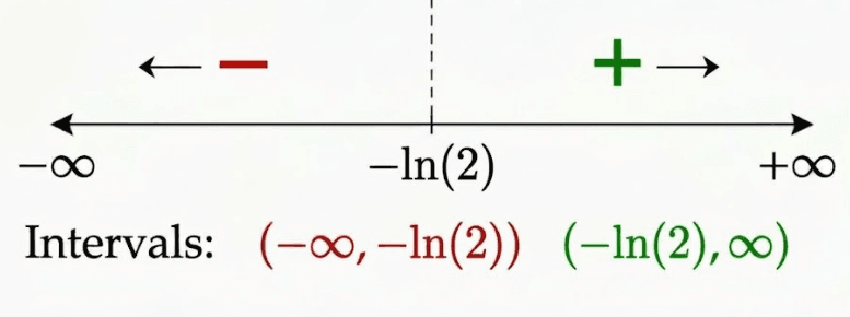
- Solve: e^{-y} = 2, hence y = -\ln(2).
Step 2: Determine the Sign of g(y)
- For y < -\ln(2), g(y) = e^{-y} - 2 > 0.
- For y > -\ln(2), g(y) = e^{-y} - 2 < 0.
Step 3: Draw the Phase-Line
Analysis:
- Stable Point: y = -\ln(2).
Graphical Illustration:
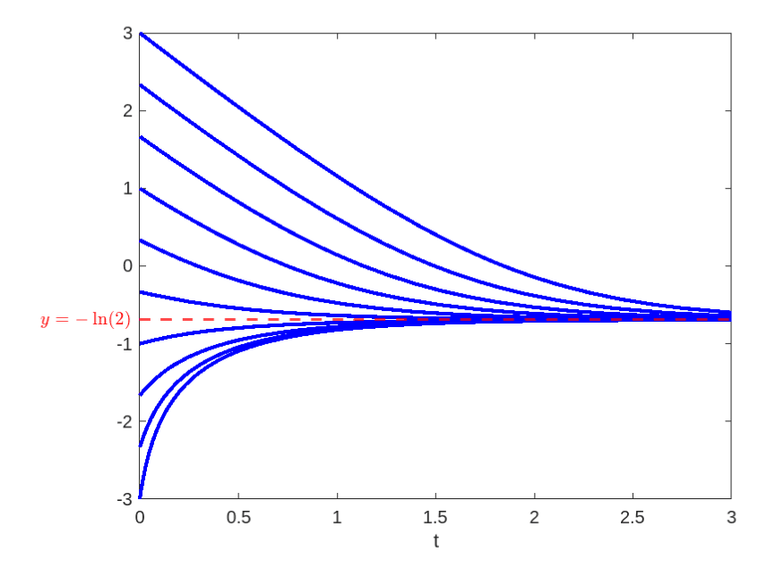
The final plot for the differential equation \frac{dy}{dt} = e^{-y} - 2 illustrates how the system evolves relative to the critical point y = -\ln(2). The plot features a horizontal dashed line at y = -\ln(2), marking the location where the rate of change \frac{dy}{dt} equals zero.
In the plot:
- For values of y less than -\ln(2), the function e^{-y} - 2 is positive, resulting in trajectories that move towards increasing values of y.
- For values of y greater than -\ln(2), the function e^{-y} - 2 is negative, causing trajectories to decrease towards -\ln(2).
1.8. Example 10: Complex Rational Function
Equation:
\frac{dy}{dt} = \frac{y^4 - 1}{y^4 + 1}
Step 1: Identify Critical Points
- Set \frac{y^4 - 1}{y^4 + 1} = 0.
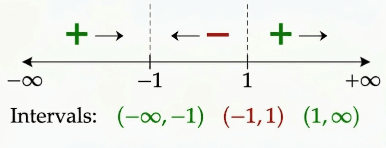
- Critical points: y = \pm 1.
Step 2: Determine the Sign of g(y)
- For y < -1, g(y) = \frac{y^4 - 1}{y^4 + 1} > 0.
- For -1 < y < 1, g(y) = \frac{y^4 - 1}{y^4 + 1} < 0.
- For y > 1, g(y) = \frac{y^4 - 1}{y^4 + 1} > 0.
Step 3: Draw the Phase-Line
Analysis:
- Stable Points: y = \pm 1 (both are semistable).
Graphical Illustration:
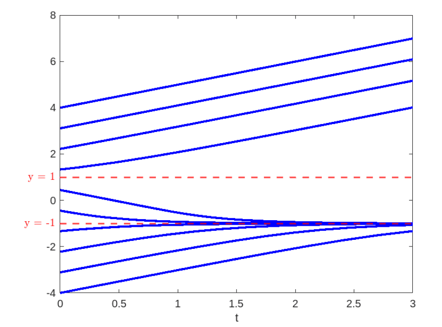
The final plot illustrates the behavior of the system governed by the differential equation \frac{dy}{dt} = \frac{y^4 - 1}{y^4 + 1}. It highlights how y changes over time for various initial conditions. Horizontal dashed lines at y = \pm 1 denote the critical points where \frac{dy}{dt} = 0.
The plot shows:
- For initial values less than -1, \frac{dy}{dt} > 0, so y increases towards y = -1.
- For initial values between -1 and 1, \frac{dy}{dt} < 0, indicating that y decreases towards y = -1 or y = 1.
- For initial values greater than 1, \frac{dy}{dt} > 0, meaning that y increases towards y = 1.
This visualization shows that y = \pm 1\ are semi stable points, with trajectories moving towards these points but not necessarily converging or diverging based on the initial conditions.
You can use MATLAB to practice and visualize graphs in more detail, helping you analyze and understand how they work. Phase-line portraits are powerful tools for understanding the qualitative behavior of solutions to autonomous differential equations.
These examples provide a variety of types of differential equations and their phase-line portraits, helping to illustrate different scenarios and behaviors of solutions. Each example includes the steps for constructing the phase-line and analyzing stability, providing a comprehensive understanding of the phase-line method.
Stay tuned for more exciting content on ODEs.
9. Phase-Line Portraits for Autonomous Equations II