Numerical methods are essential tools for approximating solutions to differential equations, especially when analytical solutions are challenging to find.
1. Introduction
Here's an example that illustrates why some problems are challenging to solve analytically and how various methods might not yield a straightforward solution:
This problem is difficult to solve analytically due to several reasons:
1. Nonlinearity: The differential equation involves an exponential function and a sine function of y, making it a nonlinear equation. Nonlinear equations often do not have closed-form solutions, and standard methods for linear ODEs cannot be applied directly.
2. Complex Function Composition: The function e^y + t^2 \sin(y) is a combination of an exponential function and a trigonometric function. The composition of these functions with y and t adds to the complexity of finding an exact solution.
Solution Methods Considered
1. Separation of Variables: This method requires the ability to separate y and t into different sides of the equation. For this problem, separating e^y + t^2 \sin(y) into different terms involving only y on one side and t on the other is not possible.
2. Integrating Factor: This technique is useful for linear differential equations. Since our problem is nonlinear, an integrating factor approach is not applicable.
3. Substitution Methods: Substitutions like y = ut can simplify certain differential equations, but in this case, substituting y = ut or other similar substitutions do not simplify the equation into a more solvable form.
4. Exact Solution Techniques: For exact solutions, we typically need the differential equation to be in a form that allows finding a general solution. This equation does not fit into such a form.
For many differential equations, particularly nonlinear ones, finding an analytical solution is not straightforward or possible. Numerical methods provide a practical approach to approximating solutions when analytical methods fall short.
Among the simplest (and least accurate) of these methods are the Euler methods. In this section, we explore the Explicit Euler Method and the Implicit Euler Method, both of which are foundational techniques in numerical analysis.
2. Explicit Euler Method
The Explicit Euler Method is a straightforward approach to solving degree-one initial value problems (IVPs) of the form:
\frac{dy}{dt} = f(t, y), \quad y(t_0) = y_0
The method is based on the definition of the derivative using difference quotients:
For small positive h, this can be approximated as:
\frac{y(t + h) - y(t)}{h} \approx f(t, y(t))
Solving for y(t + h) gives us the following iterative formula:
y(t + h) \approx y(t) + h \cdot f(t, y(t))
2.1. Mesh Points
- Suppose we want to find y(t) starting from the initial point t = t_0 and initial value y(t_0) = y_0.
- In explicit Euler, we assume t > t_0.
- So, we have an interval [t_0, T], and we divide this interval into N equal subintervals (subsections), where each subinterval will be of length h, called the step size.
h = \frac{T - t_0}{N}
- Now we can define the mesh points t_0, t_1, t_2, \ldots, t_N, where t_N = T.
- In the Euler method, we iteratively approximate the value of y at each mesh point. Starting with y(t_0) = y_0, we approximate y(t_1), then y(t_2), and so on.
- Using y(t_0) = y_0, we approximate y(t_1) as:
y(t_1) \approx y_0 + h f(t_0, y_0)
- Similarly, to approximate y(t_2), we use the value from y(t_1):
y(t_2) \approx y(t_1) + h f(t_1, y(t_1))
- This process is repeated iteratively, updating the value at each mesh point, until we approximate y(t_N), which gives the value of y(T).
If we set t = t_n, then t + h = t_{n+1} and the formula becomes:
y(t_{n+1}) \approx y(t_n) + h \cdot f(t_n, y(t_n))
This leads to the Euler method formula:
y_{n+1} = y_n + h \cdot f(t_n, y_n)
Steps to Implement the Explicit Euler Method
1. Initialize the starting values: t_0 = t_I and y_0 = y_I.
2. Iterate using the formula y_{n+1} = y_n + h \cdot f(t_n, y_n) for n = 0, 1, \dots, N-1.
3. Output the values y_n, which approximate y(t_n).
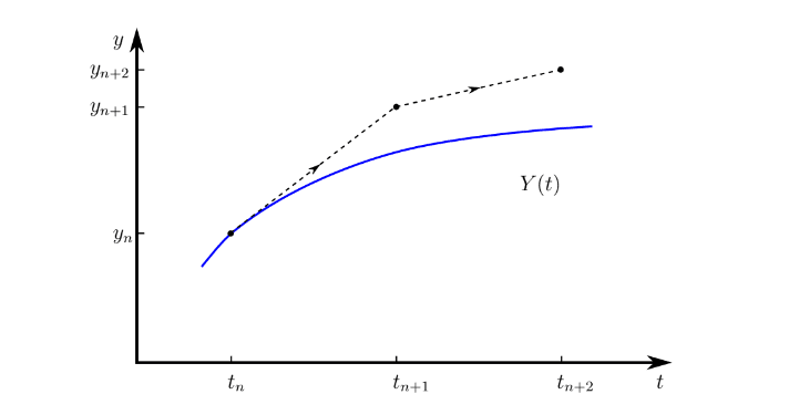
The blue line shows the actual y(t) function and the dotted line shows the y function approximated using the Euler method.
1. As it can be seen the difference between the actual y and Euler approximated y becomes larger as we go along the Mesh points.
2. The Euler method gives good approximations when t0 and T are not too far apart as seen above.
1. As it can be seen the difference between the actual y and Euler approximated y becomes larger as we go along the Mesh points.
2. The Euler method gives good approximations when t0 and T are not too far apart as seen above.
2.2. Examples:
Example 1:
Consider the problem:
\frac{dy}{dt} = -2y, \quad y(0) = 5
Using h = 0.2, approximate y(0.6).
Step 1: Initialize t_0 = 0 and y_0 = 5.
Step 2: Perform the calculations:
- f_0 = -2 \cdot 5 = -10
- y_1 = 5 + 0.2 \cdot (-10) = 3
- f_1 = -2 \cdot 3 = -6
- y_2 = 3 + 0.2 \cdot (-6) = 1.8
- f_2 = -2 \cdot 1.8 = -3.6
- y_3 = 1.8 + 0.2 \cdot (-3.6) = 1.08
Thus, y(0.6) \approx y_3 = 1.08.
Example 2:
Consider the differential equation:
\frac{dy}{dt} = t^2 + y^2, \quad y(0) = 1
We want to approximate y(0.2) using the Explicit Euler Method with step size h = 0.1.
The Implicit Euler Method is a variation of the Euler Method that, instead of using the current point to calculate the next value, involves the next point in its calculation. The derivative is approximated backward in time:
For small positive h, this can be approximated as:
\frac{y(t) - y(t - h)}{h} \approx f(t, y(t))
Solving for y(t) gives us:
y(t - h) \approx y(t) - h \cdot f(t, y(t))
Mesh point setup is the same as in the Euler method
Setting t = t_{n+1}, so t - h = t_n, we have:
y(t_{n+1}) - h \cdot f(t_{n+1}, y(t_{n+1})) \approx y(t_n)
This gives the formula for the Implicit Euler Method:
y_{n+1} - h \cdot f(t_{n+1}, y_{n+1}) = y_n
Solving the Implicit Equation
The key difference in the implicit method is that y_{n+1} is involved on both sides of the equation, meaning we must solve for y_{n+1}. This often requires numerical methods, such as the Newton-Raphson method, especially when f(t, y) is nonlinear.
3.1. Examples:
Example 1: Solving Implicitly
Consider the equation:
\frac{dy}{dt} = y + t, \quad y(0) = 1
Using h = 0.1, approximate y(0.1) using the Implicit Euler Method.
The Implicit Euler method is numerically stable because it uses information from both the current and future steps when calculating the approximation. Specifically, in the update formula:
y_{n+1} = y_n + h f(t_n, y_{n+1}),
the value y_{n+1} is used on both sides of the equation. This means that the method accounts for the present state (y_n) and also incorporates information from the future state (y_{n+1}), providing a more accurate approximation. By solving for y_{n+1}, the method handles stiff equations better and is more stable than the Explicit Euler method, which relies only on the current step to estimate the next.
The Implicit Euler method reduces numerical instability because it takes into account the anticipated behavior at the next step, which often makes it much more robust, especially when dealing with stiff equations or rapidly changing solutions. This stability is particularly valuable when larger step sizes are used.
Problem 4:
Solve the initial value problem using the Implicit Euler method:
\frac{dy}{dt} = y - t, \quad y(0) = 1, \quad h = 0.05.
We are asked to find y(0.1).
Step-by-step solution:
1. Implicit Euler equation:
y_{n+1} - h \cdot (y_{n+1} - t_{n+1}) = y_n.
2. Step 1: For n = 0, we have t_1 = t_0 + h = 0 + 0.05 = 0.05.
5. 3. Visual Comparison of Explicit Euler and Implicit Euler
In this section, we compare the performance of Explicit Euler and Implicit Euler methods for solving the differential equation
\frac{dy}{dt} = -2y, \quad y(0) = 5.
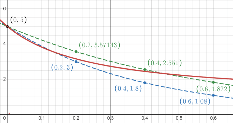
Below is a plot showing the actual solution along with the approximations obtained using both Euler methods.
The image above shows the comparison of Explicit Euler, Implicit Euler, and the exact solution.
The red line represents the exact solution y(t) = 5e^{-2t}, the blue line represents the Explicit Euler approximation, and the green line represents the Implicit Euler approximation.
As can be observed from the graph, Euler's approximations deviate more from the actual solution as t increases away from the initial value t = 0. The Explicit Euler method (blue) shows larger deviations as t increases, while the Implicit Euler method (green) tends to remain much more accurate, particularly after t > 0.3. This illustrates the improved stability of the Implicit Euler method for this type of stiff equation.
6. Error Bound in Euler's Method
In the Euler method, the error bound is typically denoted as O(h), where h represents the step size. This indicates that the error in the approximation is directly proportional to the step size. As h decreases, the error reduces, and as h increases, the error increases.
6.1. Step Size and Error Reduction
To illustrate this, consider the following:
- With a step size h, suppose the error is E.
- Reducing the step size to h/2 will approximately halve the error, resulting in an error of E/2.
This is because the Euler method is a first-order method. The global error, which accumulates over the entire interval, is proportional to h. Halving the step size doubles the number of steps, which helps to reduce the accumulation of error.
6.2. General Formula for Error
For a step size h, the global error after n steps is approximately O(h). The error is:
\text{Global Error} \approx |y(t) - y_n|
where:
- y(t) is the exact solution,
- y_n is the approximation obtained through the Euler method.
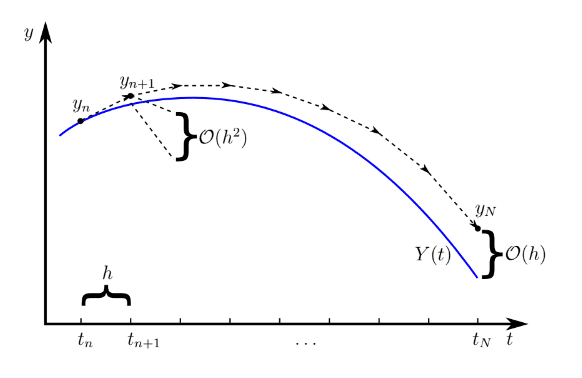
6.3. Visual Representation of Error
A graph can illustrate the difference between the actual solution curve and the Euler approximation. As the step size h decreases, the Euler approximation gets closer to the actual solution, reducing the overall global error.
6.4. Global Error in Euler’s Method
The global error in the Euler method is of order O(h). This means that if you reduce the step size, the global error decreases proportionally. For higher-order methods, such as second-order or fourth-order methods, the error reduces more rapidly with decreasing step size. For instance, a fourth-order method has a global error of O(h^4), meaning halving the step size reduces the error by a factor of 1/16.
Key Points:
- Global Error: The error accumulated over the entire interval.
- Local Error: The error at each individual step, typically of order O(h^2), but the global error accumulates as O(h).
- Higher-Order Methods: These methods provide more accuracy with smaller global errors as you reduce the step size.
6.5. Error Estimation Example
If you use the Euler method with a step size h and the error is E, reducing the step size to h/2 will result in a new error approximately E/2, demonstrating the direct relationship between step size and error.
Understanding this relationship allows you to better control the accuracy of your numerical solutions using the Euler method.